Prepare Data for Cell2Net Training on PBMC

This tutorial demonstrates the comprehensive data preparation pipeline for Cell2Net training using Peripheral Blood Mononuclear Cells (PBMC) multiome data. We’ll transform raw single-cell measurements into analysis-ready datasets optimized for regulatory network modeling.

Overview

Cell2Net requires carefully prepared multiome data that integrates:

1. Gene expression profiles (RNA-seq)

2. Chromatin accessibility (ATAC-seq)

3. DNA sequence information for regulatory regions

4. Transcription factor motif annotations

5. Peak-to-gene regulatory relationships

import warnings
warnings.filterwarnings('ignore')

import os
import numpy as np
import pandas as pd
import scanpy as sc
import mudata as md
import cell2net as cn

md.set_options(pull_on_update=False)

<mudata._core.config.set_options at 0x7fe8ebb76f60>

cn.__version__

'0.13'

Load Raw PBMC Multiome Data

Import the preprocessed PBMC multiome dataset containing paired RNA-seq and ATAC-seq measurements. This dataset represents the full cellular diversity of the peripheral blood immune system.

mdata = md.read_h5mu(f'./mdata.h5mu')

Examine the structure and dimensions of our multiome dataset:

mdata

MuData object with n_obs × n_vars = 11131 × 131516
  obs:	'cell_type', 'cell_type_v2', 'total_counts_rna', 'total_counts_atac', 'total_counts_rna_log', 'total_counts_atac_log'
  2 modalities
    rna:	11131 x 15932
      obs:	'cell_type', 'n_genes_by_counts', 'log1p_n_genes_by_counts', 'total_counts', 'log1p_total_counts', 'pct_counts_in_top_50_genes', 'pct_counts_in_top_100_genes', 'pct_counts_in_top_200_genes', 'pct_counts_in_top_500_genes', 'cell_type_v2'
      var:	'genes', 'n_cells', 'n_cells_by_counts', 'mean_counts', 'log1p_mean_counts', 'pct_dropout_by_counts', 'total_counts', 'log1p_total_counts', 'highly_variable', 'highly_variable_rank', 'means', 'variances', 'variances_norm'
      uns:	'cell_type_colors', 'cell_type_v2_colors', 'hvg'
      obsm:	'X_umap'
      layers:	'counts'
    atac:	11131 x 115584
      obs:	'cell_type', 'n_genes_by_counts', 'log1p_n_genes_by_counts', 'total_counts', 'log1p_total_counts', 'pct_counts_in_top_50_genes', 'pct_counts_in_top_100_genes', 'pct_counts_in_top_200_genes', 'pct_counts_in_top_500_genes', 'cell_type_v2'
      var:	'peaks', 'n_cells_by_counts', 'mean_counts', 'log1p_mean_counts', 'pct_dropout_by_counts', 'total_counts', 'log1p_total_counts'
      uns:	'cell_type_colors', 'cell_type_v2_colors'
      obsm:	'X_umap'
      layers:	'counts'

RNA Data Preprocessing

Apply standard single-cell RNA-seq normalization and dimensionality reduction:

1. Total count normalization: Scale gene expression to account for sequencing depth differences

2. Log transformation: Stabilize variance and make data more normally distributed

3. Principal Component Analysis: Reduce dimensionality while preserving major expression patterns

This preprocessing is essential for identifying highly variable genes and computing cellular similarities.

sc.pp.normalize_total(mdata['rna'])
sc.pp.log1p(mdata['rna'])
sc.tl.pca(mdata['rna'], n_comps=30, use_highly_variable=True)

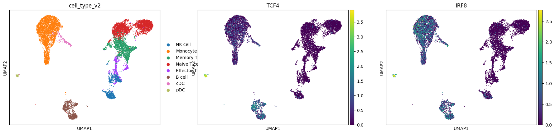
Visualize Cellular Diversity

Explore the immune cell populations and their marker gene expression patterns. This visualization helps us understand:

• Cell type distribution: Major immune populations (T cells, B cells, monocytes, etc.)

• Marker gene expression: TCF4 (B cell/pDC marker) and IRF8 (myeloid/DC marker)

• Data quality: Well-separated cell types indicate good data quality

sc.pl.umap(mdata["rna"], color=["cell_type_v2", "TCF4", "IRF8"])

Create Metacells for Network Modeling

Generate metacells to aggregate similar single cells for improved Cell2Net training:

Why Metacells?

• Noise reduction: Average out technical variability while preserving biological signal

• Computational efficiency: Reduce dataset size from ~10K cells to 1K metacells

• Statistical power: Improve signal-to-noise ratio for regulatory relationships

• Cell type preservation: Maintain representation of all immune populations

Metacell Generation Process:

1. Similarity calculation: Use PCA and nearest neighbor graphs

2. Community detection: Group similar cells using clustering algorithms

3. Expression aggregation: Average gene expression within each metacell

4. Quality control: Ensure metacells represent coherent cell states

mdata_bulk = cn.tl.get_metacells(mdata, n_metacells=1000)

Examine the metacell metadata and cell type composition:

mdata_bulk.obs

	cell_type	cell_type_v2	total_counts_rna	total_counts_atac	total_counts_rna_log	total_counts_atac_log
AAACAGCCAGTAGGTG-1	naive CD4 T cells	Naive T cell	7598.0	35084.0	3.880699	4.545109
AAACATGCAAGGTCCT-1	naive CD8 T cells	Naive T cell	3238.0	21146.0	3.510277	4.325228
AAACCAACATAATCCG-1	classical monocytes	Monocyte	7947.0	36882.0	3.900203	4.566814
AAACCGAAGTGAGCAA-1	CD56 (dim) NK cells	NK cell	1295.0	13810.0	3.112270	4.140194
AAACCGGCATAATCAC-1	myeloid DC	cDC	7216.0	25034.0	3.858297	4.398530
...	...	...	...	...	...	...
TTTGTCCCAGCTACGT-1	effector CD8 T cells	Effector T cell	4358.0	16815.0	3.639287	4.225697
TTTGTCTAGACAACAG-1	memory B cells	B cell	6463.0	39713.0	3.810434	4.598933
TTTGTCTAGAGAGCCG-1	effector CD8 T cells	Effector T cell	2749.0	23267.0	3.439175	4.366740
TTTGTGGCAGTTTGTG-1	classical monocytes	Monocyte	2165.0	18096.0	3.335458	4.257583
TTTGTTGGTCCACAAA-1	memory B cells	B cell	10103.0	8004.0	4.004450	3.903307

1000 rows × 6 columns

Check the dimensions of our metacell dataset:

mdata_bulk

MuData object with n_obs × n_vars = 1000 × 131516
  obs:	'cell_type', 'cell_type_v2', 'total_counts_rna', 'total_counts_atac', 'total_counts_rna_log', 'total_counts_atac_log'
  2 modalities
    rna:	1000 x 15932
      obs:	'cell_type', 'n_genes_by_counts', 'log1p_n_genes_by_counts', 'total_counts', 'log1p_total_counts', 'pct_counts_in_top_50_genes', 'pct_counts_in_top_100_genes', 'pct_counts_in_top_200_genes', 'pct_counts_in_top_500_genes', 'cell_type_v2'
      var:	'genes', 'n_cells', 'n_cells_by_counts', 'mean_counts', 'log1p_mean_counts', 'pct_dropout_by_counts', 'total_counts', 'log1p_total_counts', 'highly_variable', 'highly_variable_rank', 'means', 'variances', 'variances_norm'
      layers:	'counts'
    atac:	1000 x 115584
      obs:	'cell_type', 'n_genes_by_counts', 'log1p_n_genes_by_counts', 'total_counts', 'log1p_total_counts', 'pct_counts_in_top_50_genes', 'pct_counts_in_top_100_genes', 'pct_counts_in_top_200_genes', 'pct_counts_in_top_500_genes', 'cell_type_v2'
      var:	'peaks', 'n_cells_by_counts', 'mean_counts', 'log1p_mean_counts', 'pct_dropout_by_counts', 'total_counts', 'log1p_total_counts'
      layers:	'counts'

Process and Visualize Metacells

Apply dimensionality reduction to metacells for quality assessment and visualization:

1. Re-normalize: Account for aggregation effects in metacells

2. PCA: Capture main expression variation patterns

3. Neighborhood graph: Build cell similarity network

4. UMAP embedding: Create 2D visualization of metacell relationships

This processing ensures metacells maintain the biological structure of the original data while providing noise reduction benefits.

# visualize metacells
sc.pp.normalize_total(mdata_bulk['rna'])
sc.tl.pca(mdata_bulk['rna'], n_comps=30, use_highly_variable=True)
sc.pp.neighbors(mdata_bulk['rna'])
sc.tl.umap(mdata_bulk['rna'])

Validate Metacell Quality

Visualize metacells colored by cell type and marker genes to ensure:

• Cell type preservation: Each metacell maintains coherent cell identity

• Marker gene expression: Key lineage markers (TCF4, IRF8, IRF1) show expected patterns

• Spatial organization: Similar cell types cluster together in UMAP space

• Reduced noise: Smoother expression patterns compared to single cells

sc.pl.umap(mdata_bulk['rna'], color=["cell_type_v2", "TCF4", "IRF8", "IRF1"])

Add Genomic Annotations

Integrate essential genomic information for Cell2Net modeling:

1. Gene TSS Coordinates

• Extract transcription start site (TSS) positions from GTF annotation

• Define promoter regions for regulatory analysis

• Enable distance-based peak-to-gene associations

2. Peak Sequence Extraction

• Define 256bp windows around ATAC-seq peaks

• Extract DNA sequences from reference genome

• Prepare sequence data for attention mechanisms

3. DNA Sequence Integration

• Link each accessibility peak with its DNA sequence

• Enable sequence-guided regulatory modeling

• Support motif-based feature extraction

This genomic annotation is crucial for Cell2Net’s sequence-aware architecture.

cn.pp.add_gene_tss_coord(mdata_bulk, gene_gtf='../../../../data/refdata-gex-GRCh38-2020-A/genes/genes.gtf.gz')
cn.pp.add_peaks(mdata_bulk, mod_name='atac', peak_len=256)
cn.pp.add_dna_sequence(mdata_bulk, ref_fasta='../../../../data/refdata-gex-GRCh38-2020-A/fasta/genome.fa')

Load and Filter Transcription Factor Motifs

Prepare transcription factor binding site motifs for regulatory analysis:

Motif Database (JASPAR2024):

• Comprehensive collection of experimentally validated TF binding motifs

• Position weight matrices (PWMs) for sequence scanning

• Covers major transcription factor families relevant to immune cells

Gene-Based Filtering:

• Retain only motifs for TFs expressed in our PBMC dataset

• Reduces computational complexity and focuses on relevant regulators

• Ensures TF-target relationships are biologically plausible

This curated motif set enables identification of functional TF binding sites in accessible chromatin regions.

motifs = cn.pp.get_tf_motifs(database='JASPAR2024')
cn.pp.filter_motifs_by_genes(motifs, mdata_bulk)

Scan for Transcription Factor Binding Sites

Identify TF binding sites within accessible chromatin regions:

Motif Matching Process:

1. Sequence scanning: Apply TF motifs to DNA sequences of ATAC-seq peaks

2. Score calculation: Compute binding affinity scores based on position weight matrices

3. Threshold filtering: Retain high-confidence binding site predictions

4. Genomic annotation: Map binding sites to peaks and nearby genes

Output:

• Binary matrix indicating TF binding site presence/absence in each peak

• Quantitative scores for binding site strength

• Spatial relationships between TFs, peaks, and target genes

This motif matching provides mechanistic links between TF activity and chromatin accessibility for Cell2Net modeling.

cn.pp.match_motif(mdata_bulk, motifs)

Establish Peak-to-Gene Regulatory Links

Create the core regulatory network by linking accessible chromatin regions to target genes:

Peak-to-Gene Mapping Strategy:

1. Distance-based associations: Link peaks to nearby genes within reasonable genomic windows

2. Correlation analysis: Compute associations between peak accessibility and gene expression across metacells

3. Sequence-guided refinement: Use DNA sequence features to improve link predictions

4. Statistical significance: Apply multiple testing correction for robust associations

Key Parameters:

• min_n_peaks=3: Require minimum peak count per gene for reliable modeling

• highly_variable=True: Focus on genes with informative expression variation

• inplace=True: Store results directly in the MuData object

Output:

Peak-to-gene association matrix forming the foundation for Cell2Net’s attention-based regulatory modeling.

cn.pp.peak_to_gene(mdata_bulk,
                   ref_fasta='../../../../data/refdata-gex-GRCh38-2020-A/fasta/genome.fa',
                   min_n_peaks=3,
                   highly_variable=True,
                   gene_name_col="genes",
                   inplace=True)

Construct TF-to-Gene Regulatory Networks

Build transcription factor regulatory networks by integrating motif information with peak-to-gene links:

TF-Gene Network Construction:

1. Motif-peak associations: Identify which TFs have binding sites in each peak

2. Peak-gene links: Use previously computed peak-to-gene associations

3. Transitive relationships: Connect TFs to genes via their binding peaks

4. Network aggregation: Combine multiple TF-peak-gene paths into regulatory scores

Regulatory Logic:

TF → Binding Site (in Peak) → Accessible Chromatin → Target Gene Expression

Output:

• TF-to-gene regulatory network matrix

• Regulatory scores reflecting potential influence strength

• Mechanistic basis for understanding gene expression control

This network provides Cell2Net with biologically-informed priors about transcriptional regulation in immune cells.

cn.pp.tf_to_gene(mdata_bulk)

Prepare Metadata and Covariates

Consolidate essential metadata for Cell2Net training:

Key Metadata Integration:

1. Cell type annotations: Preserve immune cell population identities

2. Count statistics: Total RNA and ATAC counts per metacell for quality control

3. Cross-modal integration: Ensure consistent cell identifiers across RNA and ATAC modalities

Quality Control Metrics:

• total_counts_rna: Total gene expression per metacell (sequencing depth)

• total_counts_atac: Total accessibility counts per metacell (data quality)

• cell_type information: Biological context for model interpretation

This consolidated metadata enables Cell2Net to account for technical factors while modeling biological regulatory relationships.

df_obs_rna = mdata_bulk['rna'].obs[['cell_type', 'cell_type_v2', 'total_counts']]
df_obs_rna = df_obs_rna.rename(columns={'total_counts': 'total_counts_rna'})

df_obs_atac = mdata_bulk['atac'].obs[['total_counts']]
df_obs_atac = df_obs_atac.rename(columns={'total_counts': 'total_counts_atac'})

df_obs = pd.concat([df_obs_rna, df_obs_atac], axis=1)

mdata_bulk.obs = df_obs.copy()

Add Log-Transformed Covariates

Create log-transformed versions of count statistics for model training:

Model Covariates:

• total_counts_rna_log: Accounts for RNA sequencing depth variation

• total_counts_atac_log: Accounts for ATAC-seq technical differences

These covariates allow Cell2Net to separate technical effects from true biological regulatory relationships.

mdata_bulk.obs['total_counts_rna_log'] = np.log10(mdata_bulk.obs['total_counts_rna'])
mdata_bulk.obs['total_counts_atac_log'] = np.log10(mdata_bulk.obs['total_counts_atac'])

Save Processed Dataset

Export the fully prepared MuData object containing all components needed for Cell2Net training:

Saved Components:

• Metacell expression profiles (RNA and ATAC)

• Genomic annotations (gene TSS coordinates, peak sequences)

• Regulatory networks (peak-to-gene and TF-to-gene associations)

• Motif annotations (TF binding site predictions)

• Metadata and covariates (cell types, count statistics)

This comprehensive dataset is now ready for Cell2Net model training and regulatory network inference.

out_dir = "./02_prepare_data"
os.makedirs(out_dir, exist_ok=True)

mdata_bulk.write_h5mu(f'{out_dir}/mdata.h5mu')

Export Motif Annotations

Save transcription factor binding site predictions in standard BED format for external analysis and visualization:

BED File Contents:

• Genomic coordinates of predicted TF binding sites

• TF identity for each binding site

• Binding scores indicating prediction confidence

• Peak associations linking motifs to accessible regions

This standardized format enables integration with genome browsers, ChIP-seq validation data, and other genomic analysis tools.

# save motif match results to a bed file
motif_bed = mdata_bulk['atac'].uns['motif_match']
motif_bed.to_csv(f'{out_dir}/motif_match.bed', sep='\t', index=False, header=False)

Summary and Next Steps

✅ Data Preparation Complete:

1. Single-cell to metacells: Aggregated ~10K cells to 1K metacells for noise reduction

2. Genomic annotation: Added gene TSS coordinates and DNA sequences for all peaks

3. Motif analysis: Identified TF binding sites in accessible chromatin regions

4. Regulatory networks: Established peak-to-gene and TF-to-gene associations

5. Quality control: Prepared covariates for technical factor correction

6. Data export: Saved comprehensive dataset for Cell2Net training

🎯 Key Outputs:

• mdata.h5mu: Complete multiome dataset with all annotations

• motif_match.bed: TF binding site predictions in BED format

• Regulatory networks: Peak-gene and TF-gene association matrices

• Metadata: Cell type labels and quality control metrics

The comprehensive data preparation pipeline established here provides a robust foundation for understanding immune cell regulation through sequence-guided regulatory network modeling with Cell2Net.