Evaluating Peak-to-Gene Predictions with Experimental Validation

This tutorial demonstrates how to evaluate and compare peak-to-gene predictions from different computational methods using experimental validation data. We’ll use Hi-C and ChIA-PET datasets as ground truth to assess the quality of predicted regulatory relationships.

Overview

Computational prediction of peak-to-gene links is a fundamental challenge in single-cell genomics. To objectively compare different methods, we need experimental validation datasets that capture true regulatory relationships. This tutorial shows how to:

1. Load experimental validation data (Hi-C and ChIA-PET)

2. Compare computational predictions against experimental evidence

3. Calculate enrichment metrics to quantify method performance

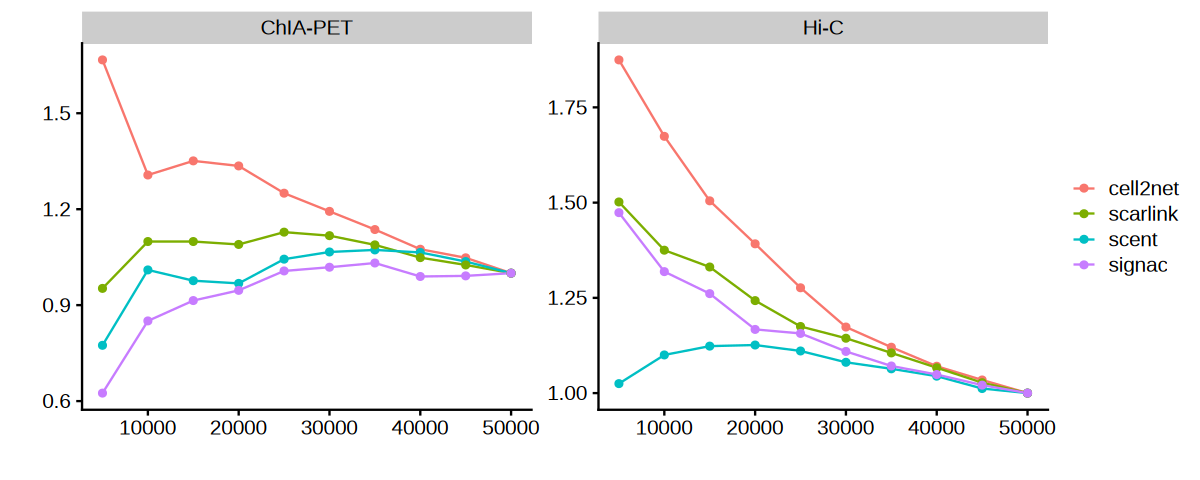
4. Visualize comparative results across multiple methods

Experimental Validation Datasets

Hi-C Data:

• Technology: Chromosome conformation capture (3C-based)

• Information: Genome-wide chromatin interactions

• Resolution: Identifies both promoter-enhancer and structural interactions

• Strength: Comprehensive, unbiased interaction mapping

ChIA-PET Data:

• Technology: Chromatin interaction analysis by paired-end tag sequencing

• Information: Protein-mediated chromatin interactions

• Resolution: Higher specificity for transcription factor-mediated loops

• Strength: Identifies functional regulatory interactions

Evaluation Strategy:

We use odds ratio analysis to measure how well each method’s top predictions are enriched for experimentally validated interactions compared to random expectations. Higher odds ratios indicate better performance in identifying true regulatory relationships.

suppressMessages(library(cicero))
suppressMessages(library(ggplot2))
suppressMessages(library(cowplot))
suppressMessages(library(gridExtra))
suppressMessages(library(dplyr))

Setup Input Directory

Define the path to processed peak-to-gene predictions from the previous tutorial (05_process_p2g).

in_dir <- "./05_process_p2g"

Load Experimental Validation Data

Import Hi-C and ChIA-PET datasets that serve as ground truth for evaluating computational peak-to-gene predictions.

Hi-C Data (ENCFF256ZMD):

• Source: ENCODE K562 Hi-C experiment

• Technology: Genome-wide chromatin interaction mapping

• Format: BEDPE (paired genomic intervals)

• Coverage: Comprehensive interaction landscape

ChIA-PET Data (ENCFF607PZX):

• Source: ENCODE K562 ChIA-PET experiment

• Technology: Protein-mediated chromatin interactions

• Format: BEDPE (paired genomic intervals)

• Specificity: Transcription factor-mediated loops

Both datasets are processed to create standardized coordinate formats matching our computational predictions.

# read Hi-C and ChIA-PET data
df_hic <- read.table("../../../../data/K562_HiC/ENCFF256ZMD.bedpe", 
                       sep = "\t", 
                       header = FALSE,
                       stringsAsFactors = FALSE)
colnames(df_hic)[1:6] <- c("chr1", "start1", "end1",
                            "chr2", "start2", "end2")

df_hic$Peak1 <- paste(df_hic$chr1, df_hic$start1, df_hic$end1, sep = "_")
df_hic$Peak2 <- paste(df_hic$chr2, df_hic$start2, df_hic$end2, sep = "_")
df_hic <- df_hic[c("Peak1", "Peak2")]

df_chiapet <- read.table("../../../../data/K562_ChIAPET/ENCFF607PZX.bedpe", 
                       sep = "\t", 
                       header = FALSE,
                       stringsAsFactors = FALSE)
colnames(df_chiapet)[1:6] <- c("chr1", "start1", "end1",
                            "chr2", "start2", "end2")
df_chiapet$Peak1 <- paste(df_chiapet$chr1, df_chiapet$start1, df_chiapet$end1, sep = "_")
df_chiapet$Peak2 <- paste(df_chiapet$chr2, df_chiapet$start2, df_chiapet$end2, sep = "_")
df_chiapet <- df_chiapet[c("Peak1", "Peak2")]

Define Evaluation Function

Create a function to compute odds ratios that measure how well computational predictions are enriched for experimentally validated interactions.

Methodology:

1. Compare predictions with validation data using genomic overlap (±100bp tolerance)

2. Calculate baseline proportion from top 50,000 predictions

3. Compute odds ratios for different prediction set sizes (5K to 50K)

4. Return enrichment metrics for performance assessment

Key Metrics:

• Proportion linked: Fraction of predictions supported by experimental data

• Odds ratio: Enrichment relative to baseline expectation

• Progressive evaluation: Performance across different stringency levels

Statistical Rationale:

Higher odds ratios indicate that a method’s top predictions are more enriched for true regulatory relationships compared to random expectations. This provides an objective measure of method performance.

compute_ratio <- function(df_pred, df_true){
    prop_list <- list()
    ratio_list <- list()
    n_links_list <- list()

    df_pred$isLinked <- compare_connections(df_pred, df_true, maxgap=100)
    df_top_50k <- df_pred %>%
        arrange(desc(score)) %>%
        slice_head(n = 50000)

    odds_b = sum(df_top_50k$isLinked) / nrow(df_top_50k)

    for(top_n in c(5000, 10000, 15000, 20000, 25000, 30000, 35000, 40000, 45000, 50000)){
        df_top <- df_pred %>%
            arrange(desc(score)) %>%
            slice_head(n = top_n)
        
        odds_a = sum(df_top$isLinked) / nrow(df_top)
        odds_ratio = odds_a / odds_b
        
        # Store results
        n_links_list <- append(n_links_list, top_n)
        prop_list <- append(prop_list, odds_a)
        ratio_list <- append(ratio_list, odds_ratio)
    }

    df_res <- data.frame(
        n_links = unlist(n_links_list),
        prop_linked = unlist(prop_list),
        odds_ratio = unlist(ratio_list)
    )

    return(df_res)
}

Evaluate All Methods Against Validation Data

Systematically evaluate each computational method (Cell2Net, SCENT, SCARlink, Signac) against both experimental validation datasets (Hi-C and ChIA-PET).

Process:

1. Load predictions from each method (processed in tutorial 05)

2. Apply evaluation function to compute odds ratios

3. Compare against both datasets for comprehensive assessment

4. Combine results into unified dataframe for visualization

5. Track method performance across different prediction set sizes

Output Structure:

• n_links: Number of top predictions evaluated

• prop_linked: Proportion supported by experimental data

• odds_ratio: Enrichment relative to baseline

• method: Computational approach name

• data: Validation dataset type (Hi-C or ChIA-PET)

df_final <- lapply(c("cell2net", "scent", "scarlink", "signac"), function(method) {
   df_pred <- read.csv(glue::glue("{in_dir}/{method}.csv"), row.names = 1)

   df_hic_res <- compute_ratio(df_pred, df_hic)
   df_chiapet_res <- compute_ratio(df_pred, df_chiapet)

   df_hic_res$method <- method
   df_chiapet_res$method <- method

   df_hic_res$data <- "Hi-C"
   df_chiapet_res$data <- "ChIA-PET"
   df <- rbind(df_hic_res, df_chiapet_res)

   return(df)
} ) %>%
    bind_rows()

Let’s examine the structure of our evaluation results:

head(df_final)

A data.frame: 6 × 5

	n_links	prop_linked	odds_ratio	method	data
	<dbl>	<dbl>	<dbl>	<chr>	<chr>
1	5000	0.05980000	1.874608	cell2net	Hi-C
2	10000	0.05340000	1.673981	cell2net	Hi-C
3	15000	0.04800000	1.504702	cell2net	Hi-C
4	20000	0.04440000	1.391850	cell2net	Hi-C
5	25000	0.04072000	1.276489	cell2net	Hi-C
6	30000	0.03743333	1.173459	cell2net	Hi-C

Visualize Method Performance Comparison

Create comprehensive plots showing how each method performs against experimental validation data.

options(repr.plot.height = 4, repr.plot.width = 10)

p <- ggplot(data = df_final, aes(x = n_links, y = odds_ratio)) +
    geom_line(aes(color = method)) +
    geom_point(aes(color = method)) +
    facet_wrap(~data, scales = "free") +
    xlab("") + ylab("") +
    theme_cowplot() +
    theme(legend.title = element_blank())

print(p)