BEAN model description
Variant and guide-level phenotypes
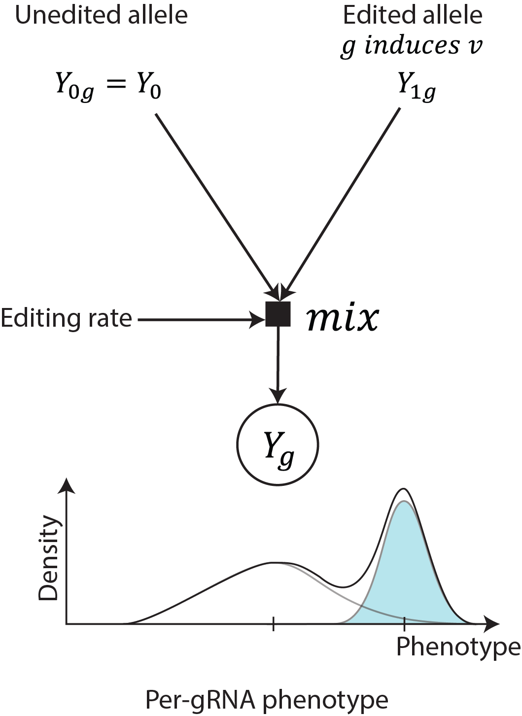
BEAN models the phenotype of cells with variant \(v,\) \(Y_{v}\) ,as normal distribution, where the wild-type cells have standard normal phenotypic distribution \(Y_{0}\) and the variant effects are quantified in a relative scale, using \(Y_{0}\) as reference.

For the cells with a guide, their phenotype is modeled as a mixture of allelic distributions produced by the guide, reflecting the heterogeneous outcome from a guide.
variant mode
In variant mode for variant screens (e.g., GWAS candidate variant
targeting library), we aggregate alleles into two categories: alleles
with (\(Y_{g1}\)) or without (\(Y_{g0}\)) the target variant.
The non-edited component in these models is fixed to have a wild-type
phenotypic distribution \(Y_0\). That is, the phenotype
\(Y_{g}\) of cells with gRNA \(g\) that induces variant
\(v\) with editing rate \(\pi\) is modeled as follows:
, where \(f_{Y_g}\) indicates the probability density function of \(Y\). The prior for \(\mu_{v}\) and \(\sigma_{v}\) are set to be narrow based on the assumption that most variant would have close to wild-type effect size of mean 0 and standard deviation 1.
Multiallelic outcome modeling in tiling mode
For saturation tiling screen, as bystander edits are more likely to have
phenotypic effect, BEAN accounts for more than one non-wild-type
allele where each allele may include one or more variants. Here, we
use the term “allele” to refer to the multiple editing outcome produced
by base editing, and we can aggregate multiple nucleotide-level variants
that lead to the same coding sequence amino acid mutations together (if
you use --translate flag in bean filter).
We denote with
\(A\left( g \right) = \{ a|\text{Allele }a\text{ is produced by }g\}\) the
set of alleles produced by gRNA \(g\) that is robustly observed
(defined by thresholds in bean-filter) The phenotype of a given
allele \(a\) is defined as the sum of phenotypic effect of
variants consisting the allele. Finally, the phenotype of cells with
gRNA \(g\) is modeled again as the mixture distribution of allelic
phenotype for the alleles it induces (\(a \in A(g)\)) as follows:
, where \(\widetilde{\pi_{a}}\) is the endogenous editing rate, estimated from \(\pi_{a}\), the reporter editing rate, of allele \(a\). The non-edited allele phenotype and the priors for \(\mu_{v}\) and \(\sigma_{v}\) are identical to the variant screen modeling.
Learning editing rate from reporter
Allele editing rates are learned from per-gRNA reporter allele counts in
pre-sort (bulk) sample (fed in as --control-condition in
bean run).
\(\mathbf{\pi}_{\mathbf{g}} = (\pi_{g0},\ \ldots,\ \pi_{g|A\left( g \right)|})\)
and per-gRNA allele count
\(\mathbf{Z}_{\mathbf{g}} = \left( A_{g0},\ \ldots,\ A_{g\left| A\left( g \right) \right|} \right)\)
are modeled as the Dirichlet and Multinomial distributions :
Where \(\mathbf{\alpha}_{\mathbf{\pi}}\) is initialized as \(\overrightarrow{\mathbf{1}}\), \(\epsilon = 1e^{- 5}\) and \(\alpha_{\text{gπ}}^{\circ}\) is the precision parameter that is fitted from the data (see Over-dispersed multinomial count data modeling). This approach partially follows DESeq2 approach of dispersion parameter estimation for the Negative Binomial distribution.
Optionally, the reporter editing rate \(\mathbf{\pi}_{\mathbf{g}}\)
can further scaled by accessibility to be used as the endogenous editing
rate \(\widetilde{\mathbf{\pi}_{\mathbf{g}}}\) through a function
\(f\), by feeding in (--scale-by-acc flag into bean run).
This function \(f\) is learned a priori from the paired reporter and
endogenous editing rate data while the deviation of
\(\widetilde{\mathbf{\pi}_{\mathbf{g}}}\) from
\(f\left( \mathbf{\pi}_{\mathbf{g}} \right)\) is fitted per gRNA.
The deviation \(\epsilon_{\text{πg}}\) below accounts for the
incomplete correlation between endogenous and reporter editing rates.
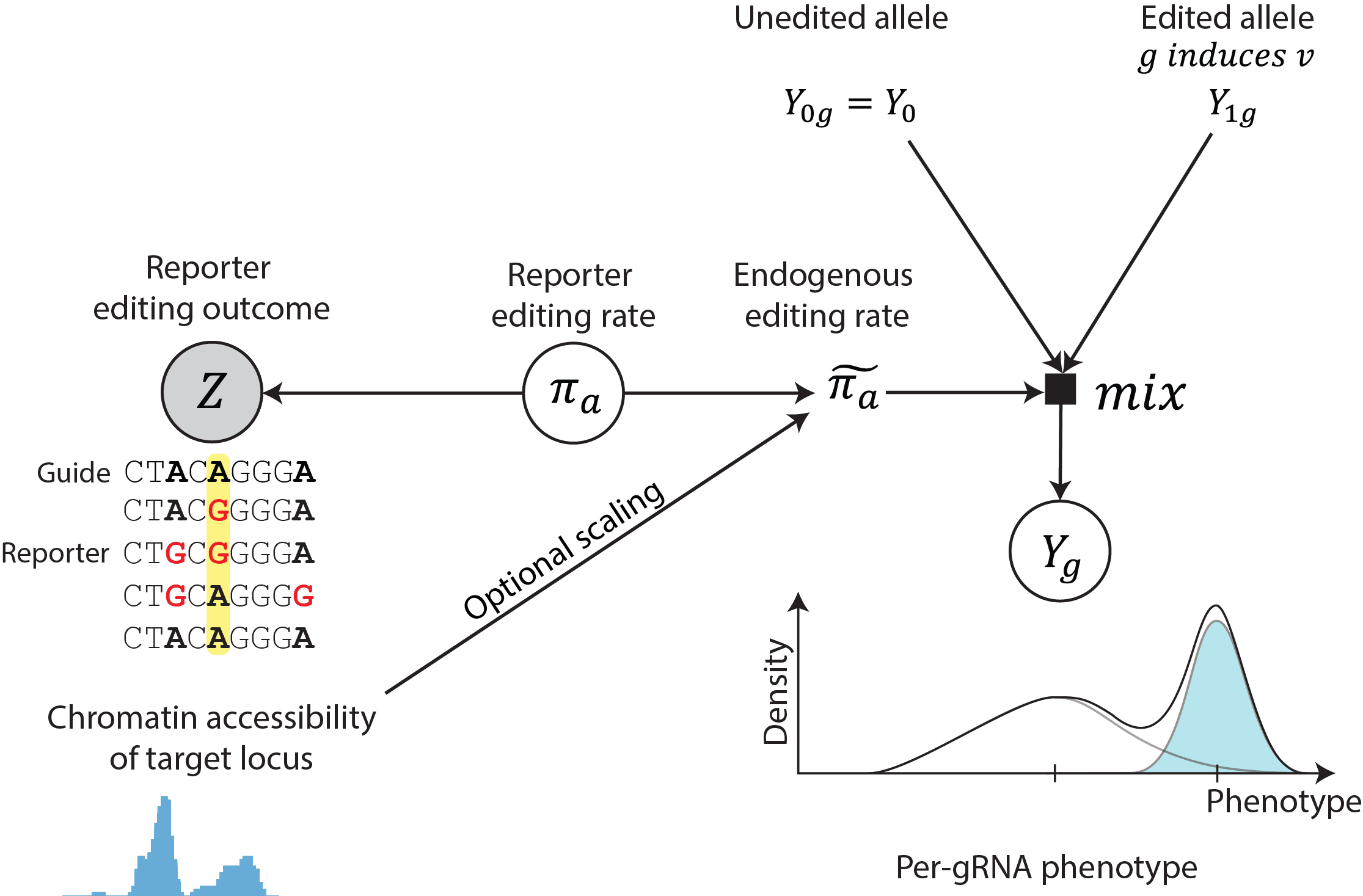
\(f\left( \pi \right)\) is fitted from the data generated for comparison of endogenous and reporter editing based on the regression \(E\left\lbrack \log\left( \frac{\pi_{\text{endo}}}{\pi_{\text{reporter}}} \right) \right\rbrack = aw + b\) where \(w\) is \(log(\text{accessibility_signal + 1})\) and the resulting coefficients \(a = 0.2513\) and \(b = \ - 1.9458\) are used for the analyses presented in this paper. The residual of the regression is fitted as the Normal distribution, which is used as the prior for the logit-scale deviation \(l_{\pi}\) (see full detail in Accessibility scaling section).
bean run without reporter
When bean run is fed with --uniform-edit, it does not require
the data to have reporter counts. In this scenario, the model assumes a
single component Normal distribution of cellular phenotype, reflecting
the assumption that all gRNAs would have the same editing efficiency.
Sorting screen model (bean run ... sorting)
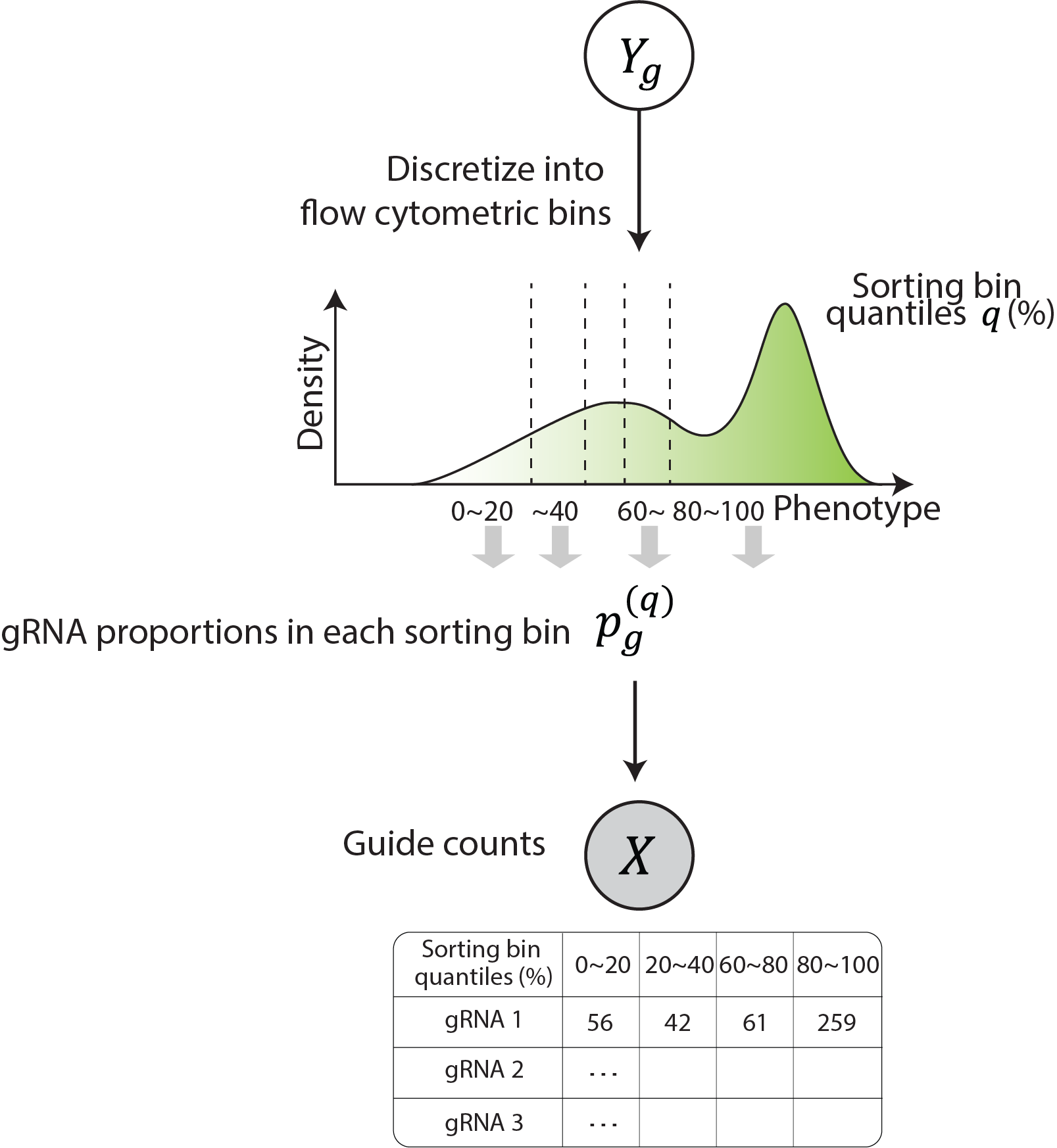
Sorting screens sorts the pool of cells with different gRNA and editing outcomes into distinct bins based on the phenotype they’re sorted on prior to sequencing. To model the sorting procedure, the proportion of cells that falls within sorting quantile bins for each gRNA is calculated analytically. This process allows for the determination of the relative fraction of cells with the gRNA that falls into each sorting bin, which is then used as the concentration parameter of Dirichlet-Multinomial distribution. Dirichlet-Multinomial distribution is chosen to model the gRNA read count across sorting bins that is over-dispersed multinomial count distribution, which we confirm from our data (see more on Supplementary Note 4 of the manuscript).
The gRNA read counts across sorting bins
and the barcode-matched gRNA read count \(\mathbf{X}_{\mathbf{\text{gr}}}^{\mathbf{b}}\mathbf{\ }\)for gRNA \(g\) and replicate \(r\) are modeled as following:
,where \(\odot\) denotes element-wise multiplication. Here, \(\mathbf{p}_{\mathbf{g}}\) is scaled as \(\mathbf{\alpha}_{\mathbf{\pi}}\) by the data-fitted precision parameter \(p_{g}^{\circ}\) (Over-dispersed multinomial count data modeling) then scaled by the sample-specific size factor \(s_r\)
where the sample size factor is calculated as in DESeq2.
For sample \(j\), \(s_{j} = \text{median}_{g}\left(\frac{X_{\text{gj}}}{\left( \prod_{v = 1}^{m}X_{\text{gj}} \right)^{1/m}} \right)\)and the same function is used to calculate size factor for barcode-matched read counts for sample \(j\), \(s_{j}^{b}\) with \(X_{\text{gj}}^{b}\).
Survival screen modeling (bean run ... survival)
Survival screen model is based on the assumption that the variant will have constant multiplicative effect by the unit time.
We will denote \(\mu_i + \mu_0\) as the relative log fold change of cell population with variant \(i\), given that the wild-type cell will have the log fold change of \(\mu_0\) as unit time passes. This is equivalent to say that the number of cells with variant \(i\) will be multiplied by \(r_i = e^{\mu_i + \mu_0}\) per unit time, whereas the number of the wild type cells will grow by \(e^{\mu_0}\).
As we observe the total gRNA abundance instead of the true variant identity in the cell, let us denote the set of well-represented alleles (including wild-type allele) induced by gRNA \(j\) as \(A_j\), and allele fraction of each allele \(a \in A_j\) as \(\pi_{j,a}\). Note that \(\sum_{a \in A_j} \pi_{j,a} = 1\) for all \(j\).
The total abundance \(p_j(t)\) of gRNA \(j\) after time \(t\) is modeled as the sum of the number of cells with allele \(a\), each proliferated by their own effect size \(\mu_a\). When an allele consists of multiple variants, we assume the additive effect (\(\mu_a = \sum_{v \in a} \mu_v\)).
To account for the fact that the allele fraction we observed at any later timepoint than \(t = 0\), we model the observed allele fractions \(\pi_{j,a}(t)\) as follows:
From the observed editing rate in time \(t>0\) \((\pi_{j,a}(t))\) and gRNA abundance in each timepoint \((p_g(t))\), we infer \(\mu_v\) and initial allele fraction \(\pi_{g,a}(0)\).
Inference
The parameters \(\mu_{v},\ \sigma_{v},\ \alpha_{\pi},\ l_{\pi}\) of posterior distributions are fitted using stochastic variational inference (SVI) using Pyro. Specifically, the posterior phenotypic distribution of each variant is fitted as a Normal distribution with a posterior standard deviation parameter and mean parameter which has Normal posterior distribution:
Where \(\mathcal{D}\) is observed data for the model and \(Q\) is the variational distribution.
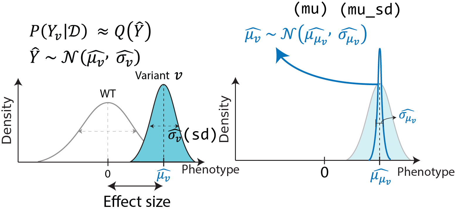
Negative control variants are used to control the significance of variant effect, by fitting the shared phenotypic distribution of negative controls as a single normal distribution. Subsequently the results are scaled so that the fitted negative control distribution is transformed to a standard normal.
In order to control for false discovery with negative control variants, the standard deviations of variants \(\sigma_{\mu_{v}}^{\left( \text{scaled} \right)}\) are scaled so that the standard deviation of \(\mu_{n}\), where \(n\) are the negative control variants, is equal to 1.
Where \(\widehat{\sigma_{n}}\) is fitted as the standard deviation estimate of \(z_{\mu_{n}}^{(scaled)} = \mu_{\mu_{n}}^{\left( \text{scaled} \right)}/\sigma_{\mu_{n}}^{(scaled)}\).
The model’s output includes various parameters relating to the phenotype
of the variant, such as the mean and standard deviation of variant
phenotype
\(\mu_{v}^{\left( \text{scaled} \right)},\ \sigma_{v}^{\left( \text{scaled} \right)}\)
and scaled and significance-adjusted phenotypic mean distribution
parameters
\(\mu_{\mu_{v}}^{\left( \text{scaled} \right)},\ \sigma_{\mu_{v}}^{\left( \text{scaled} \right)},\ \sigma_{v}^{(adj)},\ z_{\mu_{v}}^{(adj)}\)
where
\(z_{\mu_{v}}^{(adj)} = \mu_{\mu_{v}}^{\left( \text{scaled} \right)}/\ \sigma_{\mu_{v}}^{(adj)}\)
are reported together with metrics quantifying per-variant evidence
provided in the input. For `variant` mode, the mean targeting gRNA
editing rate is reported and for `tiling` mode, the number of gRNAs
covering each variant (n_guide), number of co-occurring variants that
is edited together in any of the observed alleles (n_coocc), and
effective editing rate which is calculated as
\(\sum_{g \in \{ g|g\ \text{induces}\ v\}}^{}{\sum_{a \in \{ g\ \text{induces}\ a,\ a\text{ has }v\}}^{}\frac{\widetilde{\pi_{\text{ga}}}}{\left| a \right|}}\),
are reported. The model, variational distribution and inference
procedure are available as the default options of bean-run command
of bean21 software. Specifically, BEAN-Uniform is run with
--uniform-edit and full BEAN model is run by specifying
--scale-by-acc argument.
Adjusting editing rates by accessibility with --scale-by-acc
BEAN takes account for the observation that endogenous editing rate \(\widetilde{\mathbf{\pi}}\) is roughly proportional to the reporter editing rate \(\mathbf{\pi}\) and is scaled by the loci accessibility.
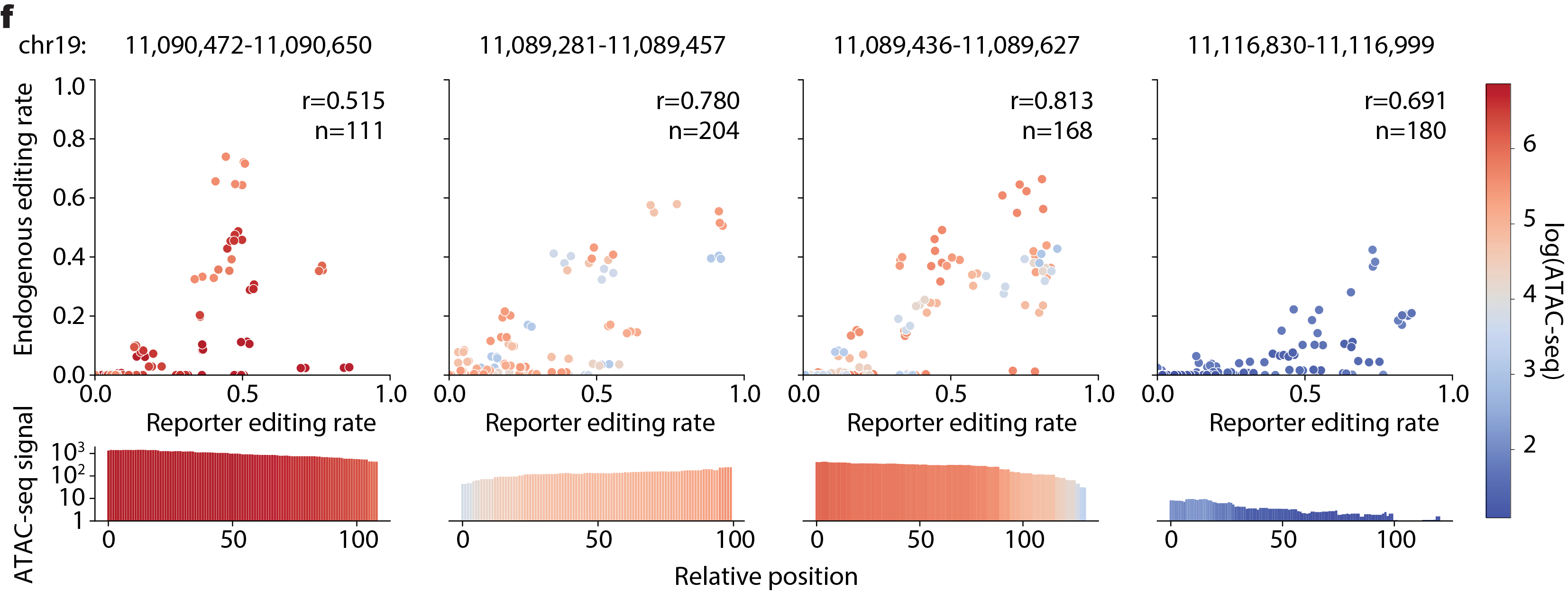
In the model, BEAN fits a function \(f\) that maps the reporter editing rate to the endogenous editing rate by assuming the proportional relationship with error \(\widetilde{\pi_{\text{gj}}} = f\left( \pi_{\text{gj}} \right) = c\pi_{\text{gj}} + \epsilon_{g}\) for non-wild-type allele \(j\) and the scaling factor \(c\) is the function of accessibility.
The scaling factor \(c\) is fitted from data by fitting the ratio between the observed nucleotide-level editing rate \(\pi_{\text{gi}}\) in reporter and endogenous target site editing rate \(\widetilde{\pi_{\text{gi}}}\) in the mini-tiling screen data. Specifically, linear model of \(r = \log\left( \frac{\widetilde{\pi_{\text{gi}}} + 0.05}{\pi_{\text{gi}} + 0.05} \right),\ \ E\left\lbrack r \right\rbrack = aw + b\) was studied where \(w = \text{window_mean}\left( \log\left( \text{accessibility_signal} + 1 \right) \right)\) and \(\text{accessibility_signal}\) is the mean log-transformed accessibility signal. The coefficients were fitted to be \(a = 0.2513,\ b = - 1.9458\) from our data and would be used as the default value.
The fitted relationship was used to transform allele editing rate in the reporter to the rate in the endogenous editing. To account for the deviation of \(r\) from the predicted, \(\epsilon_{g}\) =\(\text{logit}\left( \sum_{i \neq 0}^{}\widetilde{\pi_{\text{gj}}} \right) - \text{logit}\left( \sum_{i \neq 0}^{}\pi_{\text{gj}} \right)\) is fitted during the inference time per gRNA \(g\), and its prior is set to be \(\epsilon_{g}\mathcal{\sim N}(0,\ \sigma_{\epsilon})\) where \(\sigma_{\epsilon} = 0.655\) is the observed standard deviation of the residual \(\text{logit}\left( \widetilde{\pi_{\text{gi}}} \right) - \text{logit}\left( f\left( \pi_{\text{gi}} \right) \right)\) using the \(f\) from the above fitted relationship.
See full detail in Supplementary Notes 2.4.3 and Supplementary Figure 16 in the manuscript.
Over-dispersed multinomial count data modeling
We follow the DESeq procedure of utilizing depth-normalized sample mean and variance to fit the total concentration estimate \(\alpha_{g}^{\circ} = \sum_{k}^{}\alpha_{g}^{(k)}\) for each gRNA \(g\) and trend-fitting the concentration estimates with depth-normalized total counts, where \(\alpha_{g}^{(k)}\)is the concentration parameter of Dirichlet-Multinomial distribution \(X_{g}\ \sim\ DirMult(n_{g},\ \mathbf{\alpha =}(\alpha_{g}^{\left( 1 \right)},\ldots,\ \alpha_{g}^{(d)}))\) of a specific gRNA \(g\). Subscript \(g\) is omitted below until otherwise described for simplicity.
First, we obtain formula to estimate per-gRNA \(\alpha^{\circ}\) values using method-of-moments. For \(X = (X^{\left( 1 \right)},\ldots,\ X^{(d)})\) and \(k \in \{ 1,\ \ldots,\ d\}\),
Where \(p^{(k)} = \frac{\alpha^{\left( k \right)}}{\alpha^{\circ}}\). Given \(n\), we can get the method-of-moment estimates of \(p^{(k)}\)and \(\alpha^{\circ}\) as
Next, as multiple observations from different replicates does not share \(n\) across replicates, we follow DESeq’s count normalization procedure to obtain within-group variances and means as follows. Here, \(s_{r}^{\left( k \right)}\) is the size factor of the sample in \(r^{\text{th}}\) replicate and \(k^{\text{th}}\) sorting bin calculated as in DESeq2.
We report overdispersion of counts from comparing within-group variances and and multinomial variances. Furthermore, we observed strong linear trend between the normalized total count \(\widehat{n} = \sum_{k}^{}\widehat{\mu^{(k)}}\) and \(\widehat{\alpha^{\circ}}\) in log scale. Thus, the linear trend between \(log(\widehat{n})\) and \(log(\widehat{\alpha^{\circ}})\) is fit (See more detail in Supplementary Fig. 17 of the manuscript).
We
take\(\ {\widehat{\alpha^{\circ}}}_{\text{tr}}\left( {\widehat{n}}_{g} \right)\)
as the final \(\alpha^{\circ}\) estimate. We provide the option to
shrink the \(\widehat{\alpha_{g}^{\circ}}\) for each gRNA \(g\)
towards the trend-fitted
\({\widehat{\alpha^{\circ}}}_{\text{tr}}\left( {\widehat{n}}_{g} \right)\)
with --shrink-alpha argument of bean run that utilizes
Normal-Normal conjugacy. Specifically, we consider the trend-fitted
concentration estimate
\(\log\left( {\widehat{\alpha^{\circ}}}_{\text{tr}}\left( {\widehat{n}}_{g} \right) \right)\)
as the mean of the prior distribution of \(\kappa_{g}\), which is
the mean of the normal distribution that gives rise to the
methods-of-moment(MoM)-fitted
\(\tau_{g} = \log\left( \widehat{\alpha_{g}^{\circ}} \right)\) for
individual gRNA.
Here, \(G\) is the set of gRNAs.